http://www.chemistrymag.org/cji/2000/026027pe.htm |
Jun.14, 2000 Vol.2 No.6 P.27 Copyright |
Application study of steady-state online data reconciliation
Li Bo, Chen Bingzhen, Wang Jian, Cong Songbo(Department of Chemical Engineering, Tsinghua University, Beijing, 100084, China)
Received April 26, 2000.
Abstract The technology of steady-state
online data reconciliation is discussed in detail in this paper . New approaches of data
classifying, steady state test and gross error handling are developed with the purpose of
online performance. An industrial application to a crude oil distillation unit is also
discussed, which shows that more precise data satisfying the constraints can be available
through data reconciliation.
Keywords Online Data Reconciliation, Steady-State Test, Data Classifying, Gross
Error Handling
With the increasing use of computers in
petrochemical corporation, numerous data can be acquired and be applied for many works
such as administrative management, online process simulation, online process optimization,
process control, and so on. The effectiveness of these works are directly affected by the
reliability and validity of the process data. Unfortunately, as a result of random errors
and even sometimes gross errors caused by calibration errors and instrument malfunctions,
there are inreconciliation and incompleteness in the process data. Through data
reconciliation, more precise data satisfying the constraints such as mass balances and
energy balances will be available, the unmeasured variables can be estimated at the same
time. The approaches of data reconciliation have been presented in many works(Crowe et.
al., 1996;YuanYonggen et. al.,1996), among those there are some industrial applications of
steady state data reconciliation(Chiari et. al.,1995; Weiss et. al., 1996;). But few of
those applications are performed online mainly because of three facts: first is that after
data classifying with projection matrix method, there still probably be some unobservable
unmeasured variables to be estimated during the procedure of data reconciliation, second
is that the technique of steady state test including MTE (Narasimhan et.al., 1987) and CST
(Narasimhan et. al., 1986) methods is always limited for industrial cases because of its
specific assumption that a time period is to be selected within which the process
variables are assumed to be in steady state, and the last one is that the methods
developed for gross error handling in the existing literatures are always limited by the
spatial redundancy of the data reconciliation problem.
This paper studied steady-state online data reconciliation in detail,
the technique of completely data classifying, the method of steady state test suitable for
industrial cases and the technique of gross error handling for the cases with low spatial
redundancy are discussed. An application to a crude oil distillation unit is also given.
1. STEADY-STATE ONLINE DATA
RECONCILIATION
1.1 Basic model
With the assumptions of steady state process, credible measurements, the random
measurement errors are normally distributed with zero means and known variance/covariance,
the most common approach formulates data reconciliation as the following constrained least
squares problem:
![]() (1)
(1)
![]() (2)
(2)
In this model, the weighted sum of errors is to be minimized, subject
to the constraints encapsulated in the term F(X,U).
These constraints arise because the mass balances, energy balances and any other
performance equations must be satisfied.
1.1.1 Linear case
When the constraints are linear or almost linear, the model can be written as follows:
![]() (1)
(1)
![]() (3)
(3)
The solution is obtained by means of Lagragian multipliers, and is
given by:
![]() (4)
(4)
![]() (5)
(5)
1.1.2 Nonlinear case
When the constraints are nonlinear, the model can be written as follows by linearising the
constraints:
![]() (1)
(1)
![]() (6)
(6)
where Fx and Fu are
the Jacobin matrices of the constraint functions to the measured and unmeasured variables
respectively.
One can solve the nonlinear problem directly using successive quadratic programming
algorithm. For the purpose of performing data reconciliation online, successive
linearization programming method given by Kneepper & Gorman (Knepper &
Gorman,1980)is adopted, which calculates the reconciled values as follows:![]() (7)
(7)
![]() (8)
(8)
where X0 is the vector of measured values,Xi
is the vector of reconciled values of measured variables at the ith iteration, Xi+1
is the vector of reconciled values of measured variables at the i+1th iteration,Ui
is the vector of estimated values of unmeasured variables at the ith iteration, Ui+1
is the vector of estimated values of unmeasured variables at the i+1th iterations. D=(FxQFxT)-1。
1.2 Data classifying
Chemical process variables can be classified into four types. The measured variable
can be defined as redundant or nonredundant according to its spatial redundancy, the
unmeasured variable can be defined as observable or unobservable according to its
observability. The existences of nonredundant variables or unobservable variables will
produce a singular matrix during the procedure of data reconciliation, which will result
in that the procedure can not be completed correctly.
The most commonly used method for data classifying is of projection
matrix method presented by Crowe (Crowe et. al., 1983) which classify variables into
measured and unmeasured ones. The measured variables are reconciled and the unmeasured
variables are then estimated to complete the data reconciliation work. However, if some
unmeasured variables are unobservable, the problem of calculating the inverse of a
singular matrix still exists in the procedure of estimating the unmeasured variables.
In order to perform data reconciliation online, it is necessary to
develop a new method to classify the process data thoroughly. For this purpose, we
developed a two level transformation method based on projection matrix(Wang Jian et. al.,
1999).
1.2.1 Data classifying of unmeasured variables
In equation (3), matrix B is divided into two parts B1*
and B2*. B1* consists of the columns
linearly independent with the largest number in matrix B, B2*
consists of the other columns of matrix B.
B=[B1*|B2*]
We define P2 as the projection matrix of B2*.
In the matrix P1B, the columns having all elements zero are
corresponding to the observable unmeasured variables while the other columns are
corresponding to the unobservable ones. The matrix B can be divided into two
parts B1 and B2 corresponding to the columns having all
elements zero and other columns of P1B
respectively. The unmeasured variables then can be divided into U1
including the observable ones and U2 including the unobservable
ones.
1.2.2Data classifying of measured variables
P1 is defined as the projection matrix of P1B,
multiplying equation (3) by P1P1 will remove the term of unmeasured
variables, giving:
![]() (9)
(9)
In matrix P1P2A,
the columns having all elements zero are corresponding to the nonredundant measured
variables while the other columns are corresponding to the redundant ones.
The matrix A then can be divided into two parts A1
and A2 corresponding to the redundant variables and the nonredundant
variables respectively. The measured variables are then divided into two sets, the
redundant ones constitute X1 while the non-redundant ones
constitute X2.
1.2.3 Two level transformation method
We define the following symbols:
![]()
![]()
![]()
![]()
![]()
![]()
Equation (10) is the constraint after the first level transformation. In this equation, the unobservable unmeasured variables have been eliminated, the nonredundant measured variables have been removed from the measured data set and merged into the constant term C2, so that the observable unmeasured variables can be estimated using this equation.
The equation (9) can be rewritten as:
Equation (11) is the constraint after the second level transformation. In this equation, only the redundant measured variables are considered to be reconciled.
1.2.4 Solution for linear case after data classifying
With the two level transformed constraints using projection matrix, we can solve the data reconciliation problem as follows:
First to calculate the reconciled value of the redundant measured variables, the model is given by:
where Q is the variance/covariance matrix of redundant measured variables.
The reconciled value of the redundant variable is given by:
From equation (10), the observable unmeasured variable can be estimated as follows:
There is no more work to do with the nonredundant measured variables and the unobservable unmeasured variables.
1.2.5 Solution for nonlinear case after data classifying
For nonlinear case, after data classifying, using the successive linearization programming method, the redundant variables are reconciled by:
the observable unmeasured variables are then estimated by:
where A1 、A2 、B2 is the transformed matrixes of Fx and Fy. Fx and Fy are the Jacobin matrixes of the constraint function
1.3 Steady State Test
The methods based on statistical technique are commonly used in steady state test. For chemical engineering processes, Narasimhan et. al. ( 1986 and 1987) provided two steady state test methods based on statistical theory, they are Composite Statistical Test method (CST, Narasimhan et. al., 1986) and Mathematical Theory of Evidence method(MTE, Narasimhan et. al., 1987). All these two methods need the specific assumption that a time period is to be selected within which the process variables are assumed to be in steady state.
In fact, process variables often change disorderly, which will make it very difficult for us to determine the location of a series of successive time periods satisfying the specific assumption. Therefore these two methods are greatly limited in industrial cases.
On the purpose of performing steady state test online, this paper developed a new method based on statistic test to find a steady state in complicated industrial case(Cong Songbo, 1998). This method uses a low-pass dynamic filter to reduce the variation magnitude of dynamically changed process variables, while steady process variables will remain unaffected by the filter. Then the differences between the filtered and unfiltered data are detected. A steady state is concluded if no significant differences exist. It should be emphasized that no specific assumption mentioned above is needed. Furthermore, the time period can be selected arbitrarily, one can move the time period step by step along time axis as a moving window, specifying whether it goes into a period of steady state.
1.3.1 Algorithm description
The basic assumptions are :
a. Measurements contain only random errors varying at a relatively high frequency and are normally distributed with zero means.
b. Successive measurements are mutually independent.
c. The variance/covariance matrix of measurement errors are constant and can be estimated by process data. In fact, from assumption b, the covariance matrix is diagonal. It’s element can be used as an index representing how much change can be tolerated for a steady state.
According to these assumptions, the measurement model is given by:
where
The variables pass through a low-pass filter are
where F is the function of a low-pass filter such as one order and two order linear filter. In this paper, a one order low-pass filter is introduced with its transfer function as follows
where T is the time constant of the low-pass filter.
An offset for each variable is then available:
For a low-pass filter with its gain equal to 1, it is obvious that when the process variable is in steady state,
1.3.2 Mean-value test method
In mean-value test method, the statistic quantity is:
In statistical theory, Si is a statistical variable with normal distribution N(0,1). If the mean value of variable Si is zero, a steady state can be then concluded. The hypothesis to be inspected is:
H0 : E(Si)=0, for all i=1,2,…,p
H1 : E(Si) ¹0, for at least one i
The null hypothesis is rejected if Si >Si(a ), where Si(a ) is the test criterion at a level of significance a . For multivariable case, because the variables are mutually independent, we can transform it to a series of single-variable statistical test problem through following formulations,
where,
1.3.3 Variance test method
In this method, a steady state is concluded if the process variable does not exceed a pre-specified value (or its normal variance) at a level of significance . The variance of a process variable is used to form the statistic quantity:
In statistical theory, Ci is a statistical variable with c2 distribution. The c2 test is then taken for the following hypothesis,
H0 : Ci < C(a ), for all i=1,2,…,p
H1 : Ci > C(a ), for at least one of i
A series of single-variable test can be carried out for multivariable case through the following formulations:
where,
1.3.4 Parameter tuning
Both mean-value method and variance method have their own characteristics. The first method is suitable for cases where all the process variables possess nearly the same time constants.
If the process variables, with significantly different time constants, are included in a mean-value statistic, and the time period for detection is selected according to the longer time constant, then the variation of process variable with small time constant will be taken as a process noise. The variation at different direction from its mean value, will be canceled mutually to some extent, leading to an incorrect result. The second method will be more effective than the first one in these cases. If we don’t pay much attention to the variation with a relatively high frequency, the first method will be a good choice.
The parameter T of the low pass filter is a key factor affecting the result. If T is set too small , the difference between filtered and unfiltered data will not be significant enough to be detected. On the other hand, if T is set too large, the algorithms will not be sensitive to the change of process state. Generally speaking, T is determined according to the time constants of process variables, and is often assigned with a value of 1-2 hour for most chemical processes.
The variance/covariance matrix is unknown in both of the two methods and need to be estimated with industrial experience. In fact, the criterion C(a ) can be used as an index representing the variation range within which the process data will be taken as in steady state. This physical meaning provides an approach estimating the variance/covariance matrix. Generally, the variance can be assigned to 2-5 percent of full measurement span of the corresponding variable.
The length of time period is another parameter to be chosen. It is recommended that the length of time period should be a bit longer than the setting time for all process variables concerned. For most industrial chemical processes, the length of time period should be assigned to 1-4 hours.
1.4 Gross Error Handling
The bottleneck of data reconciliation is of gross error handling (Crowe et. al., 1996; Narasimhan et. al., 1987; Cheng Lifei, 1998; Tjoa et. al., 1991; Albuquerque et. al., 1996). The sources of gross errors include malfunction instruments, decrease of measurement precision, process leaks, non-steady state operation, mismatching model, and so on(Crowe et. al., 1996).
Many methods based on statistical technique have been developed to detect and eliminate gross errors. All these methods are based on spatial redundancy of the data reconciliation problem. Among them, global test, constraint test and measurement test or modified measurement test are most commonly used (Crowe et. al., 1996; SIMSCI, 1996).
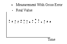
In many industrial cases, as shown in Fig. 1, gross error often occurs as the result of concurrence of measurement bias and decrease of measurement precision. It should be noted that the gross error exists not only at one measurement but at all the measurements until the instrument is adjusted, we can call this long-time existing gross error as Integral Gross Error (IGE). When we perform data reconciliation in a real plant, the common condition is that many instruments especially the flow-rate instruments have IGE, the spatial redundancy is small so that the methods mentioned above are not capable of handling the gross errors reasonably. The shortcoming of the existing methods will result in that process of data reconciliation can not be performed online. In this paper, a better new method is developed to preprocess the raw data before data reconciliation. During the data preprocessing, the sequential measurements is used to estimate the magnitudes of IGE and compensate them with a correcting coefficient.
1.4.1 Algorithm description for data preprocessing
We define the following symbols:
![]() is
the matrix of sequential measurements, where
is
the matrix of sequential measurements, where ![]() is
the vector of measured value at the time i.
is
the vector of measured value at the time i.
![]() is
the estimated matrix of unmeasured variables, where
is
the estimated matrix of unmeasured variables, where ![]() is the vector of estimated value at the time i.
is the vector of estimated value at the time i.
Let ![]() , then the vector of process variable at
time i is
, then the vector of process variable at
time i is ![]() , where n=m+u.
, where n=m+u.
For a variable ![]() with its real value
with its real value ![]() , by introducing the correcting coefficient, the
model for a bias in this variable is given by
, by introducing the correcting coefficient, the
model for a bias in this variable is given by ![]() .
.
The correcting coefficient of a measured variable represents the magnitude of bias between
its measurement and real value. The correcting coefficient of an unmeasured variable
represents the gap between its estimated value and real value.
For a system with constraints ![]() (s dimension),
the sum of the constraints residue at different time should be minimized with the
measurements corrected by the coefficients. Generally, we define an objective function
(s dimension),
the sum of the constraints residue at different time should be minimized with the
measurements corrected by the coefficients. Generally, we define an objective function ![]() representing the constraint residues. Then we can
get the correcting coefficients of variables by solving the following optimum problem:
representing the constraint residues. Then we can
get the correcting coefficients of variables by solving the following optimum problem:
 (P1)
(P1)
where, ![]() and
and ![]() are the lower-limit and the upper-limit of
correcting coefficients respectively. Generally, we set
are the lower-limit and the upper-limit of
correcting coefficients respectively. Generally, we set ![]() =0.5,
=0.5, ![]() =1.5.
=1.5.
When we use this algorithm in a linear case, P1 becomes a least square
regression problem, all the correcting coefficients are very close to the lower bounds to
reach the minimum of the objective function. However, the result is unreasonable because
it is disaccord with the basic premise of data reconciliation about credible measurements.
Considering that correcting coefficients should be close to 1, we can get the following
optimization problem with double objective functions.
This optimization problem can be solved by means of linear-weighted method with the
following transformed model:
 (P2)
(P2)
in this paper, the objective function ![]() has
the quadratic square form as follows:
has
the quadratic square form as follows:
![]()
![]()
the weights are given as follows:
![]()
With the correcting coefficient, the corrected value of measured variable is given by ![]() , most of the IGEs in that steady state have been
compensated. However, there perhaps still exist gross errors in the corrected values, we
do not get the results satisfying the constraints. Because of this, more work of data
reconciliation should be done with the following model:
, most of the IGEs in that steady state have been
compensated. However, there perhaps still exist gross errors in the corrected values, we
do not get the results satisfying the constraints. Because of this, more work of data
reconciliation should be done with the following model:
 (P3)
(P3)
where, ![]() is the vector of reconciled value of
the measured variable,
is the vector of reconciled value of
the measured variable,
![]() is
the vector of corrected average value of the measured variable,
is
the vector of corrected average value of the measured variable,![]() ,
,
![]() is
the vector of the unmeasured variable,
is
the vector of the unmeasured variable,
Q is variance/covariance matrix of the corrected value of the measured variable
P3 is the conventional least squares problem, Global Test and MIMT are used in gross error
detection and identification.
1.5 Process of steady-state online data reconciliation
In order to overcome the limits that affect the online performance of data reconciliation,
we have discussed the technique of data classifying completely, the method of steady state
test for industrial cases, and the algorithm of gross error handling for the cases having
large number of IGEs. We can summarize the process of steady-state online data
reconciliation as follows:
- Collect process data from DCS
- Steady state test, if the process is not under steady state then go to 1; else do 3
- Data classifying, calculate the spatial redundancy of that problem. If the spatial redundancy is negative, data reconciliation is not feasible, then give some advice of adding instrument, improve the precision of instruments, and so on, go to 1; else do 4
- Data preprocessing to handle the IGEs
- Solve the problem of data reconciliation, gross error detection and identification, the results satisfying the constraints then can be achieved
- Generate the result report
- Go to 1
2. APPLICATION TO A CRUDE OIL
DISTILLATION UNIT
The technique of steady-state online data reconciliation is implemented in
a crude oil distillation unit whose flowchart is shown in Fig. 2. This unit consists of 13
facilities, 37 streams. There are 74 variables to be reconciled, 67 variables including 31
flowrates and 36 temperatures are measured , 7 variables including 6 flowrates and 1
temperature are unmeasured. For nonlinear case with mass balances and energy balances, the
model of data reconciliation contains 26 equality constraints.
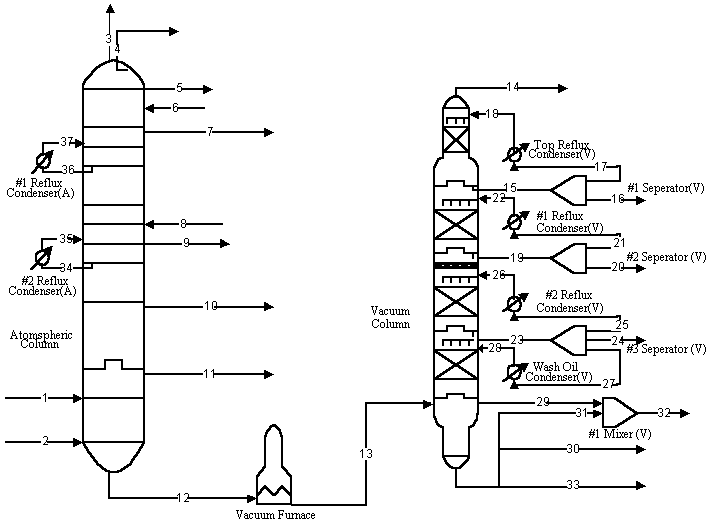
Following the process of steady-state online data reconciliation, we
perform data reconciliation using the data collected from the DCS of this unit.
1. Three variables are selected to test whether the process is under steady state. They
are: the flow-rate of crude oil, the temperature of crude oil and the top temperature of
the atmospheric column.
2. Data classifying using two level transformation method to see whether all the
unmeasured variables are observable.
3. If the process is under steady state, we use the correcting coefficient method to
handle the IGEs.
4. Global Test and MIMT are used for gross detection and identification, the data
reconciliation problem P3 is solved using equation (13)-(16).
5. Generate the result report.
Table 1 shows the reconciled result of data collected within a steady
state 2 hours long. The first column is the name of the stream in the flowchart, the
second column is the description of the stream. In the third column, the measured value
and the reconciled result of the flow-rates are shown in the first two sub-columns, the
variable type according to the result of data classifying and gross handling is shown in
the third sub-column, the percentage variance reduction is shown in the fourth sub-column.
The same items of temperature are shown in the fourth column.
Table 1 The Result of Online Data Reconciliation Within A Steady-State 2 hours long
| Stream No | Stream Description |
Flowrate(kg/hr) |
Temperature(℃) |
||||||
MV |
RV |
VT |
PVR(%) |
MV |
RV |
VT |
PVR (%) |
||
St1 |
Crude Oil (A) |
339168 |
349631 |
MR |
71.37 |
362.263 |
362.241 |
MR |
43.72 |
St2 |
Stripping Steam (A) |
2800 |
2800.57 |
MR |
0.49 |
449.745 |
449.745 |
MR |
0.00 |
St3 |
Top Reflux Draw (A) |
29920.7 |
29837.4 |
MR |
1.49 |
105.086 |
105.087 |
MR |
0.10 |
St4 |
Top Steam (A) |
3012.2 |
3011.5 |
MR |
0.27 |
105.086 |
105.086 |
MR |
0.00 |
St5 |
Top Product (A) |
6746.03 |
6664.94 |
MR |
0.25 |
105.086 |
105.086 |
MR |
0.01 |
St6 |
Top Reflux (A) |
29920.7 |
30007 |
MR |
6.32 |
74.7745 |
74.7731 |
MR |
0.15 |
St7 |
#1 Side Draw (A) |
5640.33 |
5605.12 |
MR |
0.16 |
130.727 |
130.728 |
MR |
0.00 |
St8 |
#2 Stripping Steam(A) |
212.204 |
212.208 |
MR |
0.00 |
449.745 |
449.745 |
MR |
0.00 |
St9 |
#2 Side Draw (A) |
25496.7 |
24606.5 |
MR |
1.65 |
213.089 |
213.09 |
MR |
0.13 |
St10 |
#3 Side Draw (A) |
24491.2 |
23620.9 |
MR |
0.43 |
305.015 |
305.017 |
MR |
0.15 |
St11 |
#4 Side Draw (A) |
11322.1 |
11150.7 |
MR |
0.055 |
346.102 |
346.103 |
MR |
0.04 |
St12 |
Residue (A) |
------- |
278154 |
UO |
------- |
354.486 |
355.998 |
MR |
55.31 |
St13 |
Feed Oil (V) |
------- |
278154 |
UO |
------- |
373.638 |
375.009 |
MR |
47.18 |
St14 |
Top Off Gas (V) |
162.911 |
162.88 |
MR |
0.00 |
52.4186 |
52.4178 |
MR |
0.00 |
St15 |
#1 Side Draw (V) |
------- |
61104.7 |
UO |
------- |
135.772 |
135.732 |
MR |
46.37 |
St16 |
#1 Side Product (V) |
26947.9 |
26416.5 |
MR |
15.08 |
135.772 |
135.583 |
MR |
7.15 |
St17 |
Top Reflux (V) Draw |
36022.1 |
34688.3 |
MR |
52.76 |
135.772 |
135.845 |
MR |
24.48 |
St18 |
Top Reflux (V) Back |
36022.1 |
34688.3 |
MR |
52.76 |
37.9067 |
37.865 |
MR |
12.57 |
St19 |
#2 Side Draw (V) |
------- |
85599.9 |
UO |
------- |
260.936 |
260.835 |
MR |
45.34 |
St20 |
#2 Side Product (V) |
41597.9 |
39113 |
MR |
13.63 |
260.936 |
260.617 |
MR |
8.35 |
St21 |
#1 Reflux (V) Draw |
50010.3 |
46486.9 |
MR |
57.91 |
260.936 |
261.019 |
MR |
20.48 |
St22 |
#1 Reflux (V) Back |
50010.3 |
46486.9 |
MR |
57.91 |
138.603 |
138.579 |
MR |
9.81 |
St23 |
#3 Side Draw (V) |
------- |
188169 |
UO |
------- |
314.555 |
314.494 |
MR |
51.33 |
St24 |
#3 Side Product (V) |
41566.2 |
40726.8 |
MR |
5.181 |
314.555 |
314.16 |
MR |
2.89 |
St25 |
#2 Reflux (V) Draw |
121288 |
118199 |
MR |
48.80 |
314.555 |
314.592 |
MR |
28.08 |
St26 |
#2 Reflux (V) Back |
121288 |
118199 |
MR |
48.80 |
236.314 |
236.315 |
MR |
18.32 |
St27 |
Wash Oil (V) Draw |
29995.5 |
29242.2 |
MR |
29.69 |
314.555 |
314.56 |
MR |
29.69 |
St28 |
Wash Oil (V) Back |
29995.5 |
29242.2 |
MR |
29.69 |
311.555 |
311.56 |
MR |
29.48 |
St29 |
#4 Side Draw (V) |
14230.1 |
12495.4 |
ME |
0.31 |
364.566 |
364.434 |
MR |
0.12 |
St30 |
Bitumen Residue (V) |
40000 |
39861.7 |
MR |
2.08 |
369.836 |
369.414 |
MR |
1.23 |
St31 |
VRDS Residue (V) |
------- |
118228 |
UO |
------- |
369.836 |
368.584 |
MR |
11.39 |
St32 |
VRDS (V) |
150503 |
130723 |
ME |
39.84 |
------- |
368.349 |
UO |
------- |
St33 |
Tank Residue (V) |
1283.98 |
1149.71 |
ME |
0.00 |
369.836 |
369.824 |
MR |
0.00 |
St34 |
#2 Reflux (A) Draw |
50141.5 |
50141.5 |
MR |
60.48 |
274.061 |
274.061 |
MR |
9.86 |
St35 |
#2 Reflux (A) Back |
50141.5 |
50141.5 |
MR |
60.48 |
125.578 |
125.578 |
MR |
6.45 |
St36 |
#1 Reflux (A) Draw |
48576.9 |
48576.9 |
MR |
44.71 |
156.4 |
156.4 |
MR |
19.13 |
St37 |
#1 Reflux (A) Back |
48576.9 |
48576.9 |
MR |
44.71 |
76.6044 |
76.6044 |
MR |
14.29 |
Note: MV Measured Value RV Reconciled Value VT Variable
Type
PVR Percentage Variance Reduction MR Measured Redundant Variable
UO Unmeasured Observable Variable ME Measured Variable having Gross Errors
The streams with (A) in their description enter or leave from the atmospheric column
The streams with (V) in their description enter or leave from the vacuum column.
2.1 Data classifying result
Since we use correcting coefficient method to compensate the IGEs in the measurements
instead of eliminating them from the set of measured variables, the variable type does not
change after data preprocessing. No more gross error found using the Global Test and MIMT
method which result in that all the measured variables are redundant while all the
unmeasured variables are observable after data classifying using two level transformation
method. The fact that no unobservable variable exist makes it possible to perform data
reconciliation online.
2.2 Handling the IGEs
From the variable type, the flow-rate of #4 side draw of the vacuum column, the flow-rate
of VRDS stream and the flow-rate of vacuum residue to the tank are concluded having IGEs.
The same conclusion is reached by the experienced operator. These three IGEs are
compensated with the magnitudes in accord with the operating experience.
2.3 The reliability of reconciled result
We compare the reconciled value with the result of tank scaling. In this unit, the #2 side
draw and the #3 side draw of the atmospheric column are mixed together and enter the same
tank, which is scaled once every 8 hours. The result of tank scaling including the 2 hours
within which data reconciliation is performed is 386t with the average value is
48250kg/hr, while the reconciled values of #2 side draw and #3 side draw are summed to be
48227.4kg/hr. The relative error between these two results is only 0.05%, which shows the
reliability of the result.
3. CONCLUSION
The technique of steady-state online data reconciliation
is studied in detail in this paper. With the purpose of online performance, two level
transformation method is developed to classify process variables thoroughly, new algorithm
including mean-value test method and variance test method is presented to avoid the
specific assumption which is necessary to the MTE and CST method, we also handle Integral
Gross Errors through data preprocessing using correcting coefficient method which can
overcome the limitation of the spatial redundancy to the existing methods. An industrial
application to a crude oil distillation unit is also discussed. The reconciled result is
validated by comparing with the result of tank scaling, the variance reduction after data
reconciliation is also shown. We can conclude from the result that more precise data
satisfying the constraints can be achieved through data reconciliation and can be applied
for works such as administrative management, online process optimization, and so on.
REFERENCES
[1] Crowe C M. J. Proc. Cont., 1996, 6 (2/3): 89-98.
[2] Yuan Y G, Li H S. The Technique of Data Reconciliation For Process Measurements,
China, 1996.
[3]Bussani G, Chiari M, Grottoli MG et al. Computers Chem. Engng, 1995, 19 (Suppl.):
S299-S304.
[4]Weiss G H, Romagnoli J A, Islaw K A. Computers Chem. Engng, 1996, 20 (12): 1441-1449.
[5]Knepper J C, Gorman J W. AIChE J., 1980, 26 (2): 260-264.
[6]Crowe C M, Hrymak A, Garcia C G. AIChE J., 1983, 29 (6): 881-886.
[7]Wang J, Chen B Z, He X R. Petroleum Processing and Petrochemicals (China), 1999, 30
(6):56-60.
[8]Narasimhan S, Mah R S H, Tamhane AC et al. AIChE J., 1986, 32 (9): 1409-1418.
[9]Narasimhan S, Kao C S, Mah R S H. AIChE J., 1987, 33 (11): 1930-1932.
[10]Cong S B. Postdoctoral Thesis, Dept. of Chem. & Eng. Tsinghua Univ., China, 1998.
[11]Narasimhan S, Mah R S H. AIChE J., 1987, 33 (9): 1514-1521.
[12]Cheng L F. Baccalaureate Thesis, Dept. of Chem. & Eng. Tsinghua Univ., China,
1998.
[13]Tjoa I B, Biegler L T. Computers Chem. Engng., 1991, 15 (10): 679-690.
[14]Albuquerque J S, Biegler L T. AIChE J., 1996, 42 (10): 2841-2856.
[15]DATAcon Keyword Input Manual, SIMSCI, 1996.