Estimating of baseline in capillary electrophoresis signals

1 INTRODUCTION  
Capillary electrophoresis ( CE ) is routinely used for analysis in a wide area^[1]. It has been proved to be an excellent technique for the separation of mixtures with a high separation efficiency, fast analysis time and low consumption of reagents and samples. However, the signals obtained from CE often include drifting baselines, resulting in the obscuration of useful information, changes of peak's shape and large errors as the calculation of peak areas. Thus, accurate analysis on the qualitative or quantitative test would be limited with drifting baselines. In order to improve the baseline data, a baseline subtraction technique is employed by the separation of the peaks and baselines.
    However, such baseline processing method has not been found in the previous literatures. Also, no techniques about baseline processing for CE signals have been reported. Wavelet has been put forward only in a short time, but it has become a hot topic in different areas quickly owing to its excellent characters^[2]. Wavelet as a high performance signal processing technique leads to new methods for signal processing. It has begun to be applied in analytical chemistry for signal treatment in recent years^[3]. On the baseline extracting, a valuable approach using wavelet^[4], which has been reported to be used in HPLC, divides the signal into high frequency and low frequency regions. The low frequency region is regarded as the baseline. But when it was applied to CE signal treatment, the baseline would be found to be distorted because there is no distinct boundary between the baseline's frequency and the peak's frequency. Thus, to develop a technique for baseline subtraction is urgent and useful for CE signal treatment.
    In this paper, we will describe a newly developed method using wavelet technique, named threshold fitting technique ( TFT ). TFT adopts threshold to remove peaks in signals and uses least square fitting with Mexican Hat wavelet to obtain smooth baselines. TFT can subtract baseline accurately from CE signal even when it has high noise.

2 THEORY        
The base of TFT is curve fitting. The principle of curve fitting is introducing a new function f(x) - fitting function, to approximate the original signal points which are a series of discrete data points . During the course of fitting, a criterion called least square must be followed. The least square makes the sum square of errors between the new function and the original data points to be minimum. That is
minimize          ( 1 )
where and are the ith point on the original signal and the fitting function respectively, k is the number of signal points, is the weight coefficient which always equals to 1 in this paper. The function f(x) is called as the useful signal extracted from the original one.
    Fitting function is a key of curve fitting. Here, Mexican Hat wavelet^[5]
( 2 )
is applied in the fitting function. It has a simple explicit expression and a smooth figure. The value of Mexican Hat wavelet function reduces rapidly with the coefficient. It is like the same characteristic with human watch in space. With this reason, Mexican Hat wavelet is suitable as a fitting function.
    When the original CE signal, which has a typical form shown as Fig. 1 at curve a, is fitted by Mexican Hat wavelet followed least square criterion, it is found that the fitted result (see Fig. 1 at curve b ) does not agree with the original signal well on the whole curve. They show an agreement during the segments where the curve varies slowly, those are the regions between signal peaks. But, at the sharp peak regions, the fitting result departs strongly from the original curve and the peaks become much lower and wider as shown in Fig. 1. According to the above theory, the fitting technique leads to a smooth and slowly changing curve as the result of considering all the points on the whole curve. At the peak regions, a few points are away from the majority of points, so the fitting curve will not pass through these disparate points. But those points do take part in the fitting, so the fitting curve will protuberate to the direction of peaks in virtue of the peaks' influence. Therefore, the fitting curve forms lumps at the peak regions ( those are the segments where peaks add to the baseline), but it can accord with the original signal at other regions ( those are the segments contain the baseline only ).
    In order to obtain an even and exact baseline, the primary task is to eliminate the pumps at the peak regions. In estimating the baseline, the points on the signal curve that lie on top of peaks can be considered as outliers, and thus one can imagine using a technique to subtract a baseline by ignoring those points that lie on peaks. Therefore threshold is introduced. Fixed threshold requires judgement by the operator ( which may introduce bias ) and sometimes it is impossible to find a right threshold in advance. Threshold in TFT is decided by the arithmetic automatically and achieved gradually.

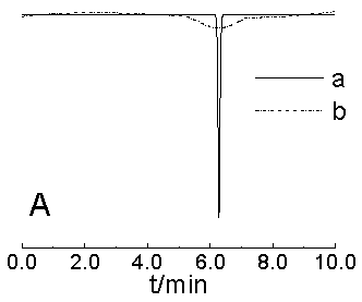
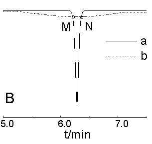
Fig. 1 Signal and its fitted curve
a. simulated CE signal b. fitted curve of a
Fig. 1(B) is a part of Fig.1( A) after magnified. M and N are the cross points of curve a and b.

3 EXPERIMENTAL
3.1 Reagents  
Roxithromycin dispersible tablets, MeOH/formamide ( 50/50 v/v ), supporting electrolyte: 10mmol/LNH₄AC-2mmol/LHAC.
3.2 Apparatus  
High performance capillary electrophoresis with amperometric detection system, Spellman High Voltage Electronics Corporation ( CZESOPN 10MCNZ2 ) were employed. The electrodes were platinum electrodes. A micro computer was used to process the data.
3.3 Data processing
All the data processing can be performed with our self-written program. During the course, the threshold changes and reaches the ideal values step by step.

4 RESULTS AND DISUSSION  
Fig. 2-D shows a peak of simulated CE signal, Fig. 3-B shows a peak of experimental CE signal. From the figures we can see that the signals have drifting baselines, so that the calculation of peak areas will meet much difficulty, such as how to find the starting point and the end-point of each peak, how to deduct the blank value at the peak regions. But if we can estimate the baselines and extract them from the original signals, all the difficulty will be solved.
4.1 The processing of simulated signals       
As a new technique, simulated signals are processed at first to test TFT's performance. We have simulated the signals with different kinds of baselines. Each result of subtracted baselines was satisfactory.
    Fig. 2-A is an example of simulated signal which is composed of two peaks and a beeline as baseline. Its estimated baseline is shown in the same figure. It is shown that the baseline is estimated accurately. Fig. 2-B is another simulated signal whose baseline is a sine wave. The result of TFT ( Fig. 2-B at curve b ) tallies completely with the theoretical baseline.
    When signals synthesized by peaks with different numbers, different positions, different heights, different widths and the same baselines are processed , the estimate baselines are still shown to be the same. It indicates that the results are not affected by the outliers ( the peaks ) .

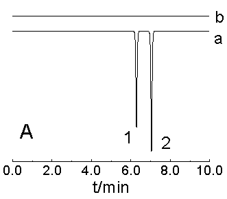a. original signal whose baseline is a beeline; b. estimated baseline	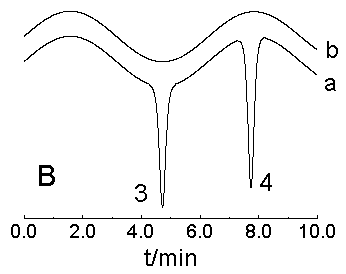a. original signal whose baseline is a sine wave;      b. estimated baseline
a. original signal with noise; (S/N=1)   b. estimated baseline	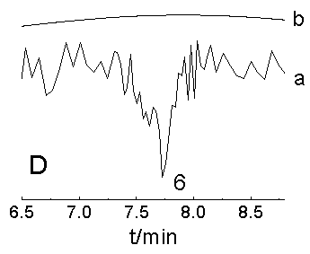Fig. D is a part of Fig. C after magnified.

Fig. 2 Simulated signals


    Then random noise produced by the computer is added to the original signals to make the simulation more like the actual situation, which always has white noise. Fig. 2-C shows an example of CE signals with noise, and it was produced by adding noise to the signal in Fig. 2-B. The result is still perfect. Experiments testify that even there is great noise on the original signals, the precise baselines without noise can be subtracted by TFT fast and no pretreatment is needed. Thus TFT is shown with great ability to deal with noise.
    Table 1 lists the theoretical values of peak height and peak area of the signals in Fig. 2. The calculated values of those signals after subtracted the baselines are listed for comparing. We can see the errors are very small. These numerals effectively prove that the estimated baselines are true.

Table 1 The relative errors of peak height and peak area

		Fig. A		Fig. B		Fig. C
		Peak 1	Peak 2	Peak 3	Peak 4	Peak 5	Peak 6
Peak height	Theoretic value	96	120	96	120	96	120
	Calculated value	96	120	95.74	119.63	95.83	119.58
	Relative error (%)	0	0	-0.27	-0.31	-0.18	-0.35
Peak area	Theoretic value	7.167	8.959	26.03	32.54	26.03	32.54
	Calculated value	7.166	8.958	25.80	32.22	25.86	32.19
	Relative error (%)	-0.01	-0.01	-0.88	-0.98	-0.65	-1.08

4.2 The processing of experimental signals           
The experimental CE signals from the detector were transferred to the computer for processing.
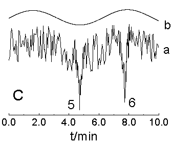
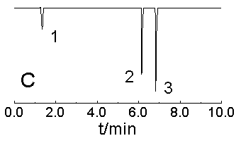
    The case of processing experimental CE signal is shown in Fig. 3. The signal of roxithromycin contains noise and the baseline is not clear. But the estimated baseline is smooth and accords well with the original signal.
    For a noisy signal, TFT can be used directly to get a slick baseline, which is significant for the analysis. But in order to obtain accurate information, we must remove the noise as well as deducting the drifting baseline. So a de-noising technique called MWLS^[6] is employed. The two techniques are combined in the program to remove the baseline and the noise at the same time. Fig. 3-C is a result of a CE signal processed by a designed program. The processed signal is distinct and the contained information is clear. We measured the peaks of the processed signal and listed the results in Table 2. After processed, the signal is much more easy for analysis and the result will be more reliable.

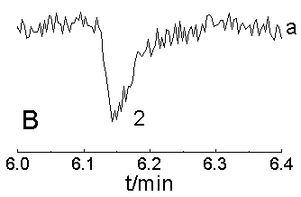a. capillary electropherograms of Roxithromycin; b. estimate baseline	Fig. B is a part of Fig. A after magnified.
The result after subtracting the baseline.	Fig. 3 Experimental CE signal

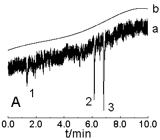
Table 2 The quantitative results of experiment signal

	Peak 1	Peak 2	Peak 3
Peak position (min)	1.35	6.15	6.82
Peak height	20.86	66.10	82.66
Peak area	1.56	3.11	4.33

5 CONCLUSION          
TFT does provide a powerful technique for estimating baseline of CE signals. It is very simple and easy to apply in the treatment of CE signal, it avoids the intervention from operators and the results are accurate. In addition, TFT is not tailed for specific data sets, it can be applied in many kinds of signals of analytical chemistry to subtract the baselines. That will make the analyses more precise.

REFERENCES             
[1] Altria K D. J. Chromatogra. A, 1999, 856: 443.
[2] Bjorn K A, Andrew M W, Douglas B K. Chemometrics and Intelligent Laboratory Systems, 1997, 37: 215.
[3] Ehrentreich F. Anal Bioanal Chem, 2002, 372: 115.
[4] Pan Z X, Shao X G, Zhong H B et al. Chinese Journal of Analytical Chemistry ( Fenxi Huaxue ), 1996, 24: 149.
[5] Yang F S. The engineering analysis and application of the wavelet transform ( Xiaobo Bianhuan De Gongcheng Fenxi Yu Yingyong ). Beijing: Scientific Press, 1999: 22.
[6] Wang Y, Mo J Y. Computers and Applied Chemistry ( Jisuanji Yu Yingyong Huaxue ), 2002, 19 (3): 379. 　

　

[ Back ] [ Home ] [ Up ] [ Next ]Mirror Site in USA  Europe  China  GBNet